2. Describing Data with Tables and Graphs
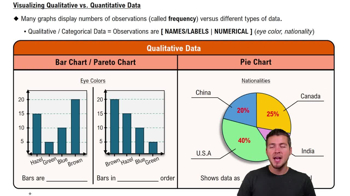
Visualizing Qualitative vs. Quantitative Data
Problem 10.3.9
Textbook Question
Interpreting a Computer Display
In Exercises 9–12, refer to the display obtained by using the paired data consisting of weights (pounds) and highway fuel consumption amounts (mi/gal) of the large cars included in Data Set 35 “Car Data” in Appendix B. Along with the paired weights and fuel consumption amounts, StatCrunch was also given the value of 4000 pounds to be used for predicting highway fuel consumption.

Testing for Correlation Use the information provided in the display to determine the value of the linear correlation coefficient. Is there sufficient evidence to support a claim of a linear correlation between weights of large cars and the highway fuel consumption amounts?
 Verified step by step guidance
1
Step 1: Identify the linear correlation coefficient (R) from the display. The value of R is provided as -0.78762826. This coefficient measures the strength and direction of the linear relationship between the weights of large cars and their highway fuel consumption.
Step 2: Interpret the value of R. Since R is negative, it indicates an inverse relationship, meaning as the weight of the cars increases, the highway fuel consumption tends to decrease. The magnitude of R (close to -1) suggests a strong linear relationship.
Step 3: Determine the significance of the correlation. To test if the correlation is statistically significant, you would typically use a hypothesis test for the correlation coefficient. The null hypothesis states that there is no linear correlation (R = 0), while the alternative hypothesis states that there is a linear correlation (R ≠0).
Step 4: Use the sample size (n = 12) and the value of R to calculate the test statistic for the correlation coefficient. The formula for the test statistic is t = R * sqrt((n - 2) / (1 - R^2)). This test statistic can then be compared to the critical t-value from the t-distribution table with degrees of freedom df = n - 2.
Step 5: Based on the test statistic and the critical t-value, determine whether to reject the null hypothesis. If the test statistic exceeds the critical value, there is sufficient evidence to support the claim of a linear correlation between weights of large cars and highway fuel consumption.
Verified video answer for a similar problem:This video solution was recommended by our tutors as helpful for the problem above
Video duration:
5mWas this helpful?

 4:39m
4:39mWatch next
Master Visualizing Qualitative vs. Quantitative Data with a bite sized video explanation from Patrick
Start learning