6. Normal Distribution and Continuous Random Variables
Standard Normal Distribution
Problem 5.1.60d
Textbook Question
Uniform Distribution A uniform distribution is a continuous probability distribution for a random variable x between two values a and b (a<b), where (a ‚ȧ x ‚ȧ b) and all of the values of x are equally likely to occur. The graph of a uniform distribution is shown below.
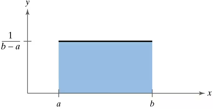
The probability density function of a uniform distribution is

on the interval from (x=a) to (x=b). For any value of x less than a or greater than b, y=0 . In Exercises 59 and 60, use this information.
For two values c and d, where a ‚ȧ c < d ‚ȧ b, the probability that x lies between c and d is equal to the area under the curve between c and d, as shown below.
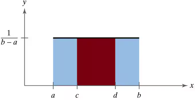
So, the area of the red region equals the probability that x lies between c and d. For a uniform distribution from (a=1) to (b=25) , find the probability that
d. x lies between 8 and 14.
 Verified step by step guidance
1
Step 1: Understand the uniform distribution. A uniform distribution is a continuous probability distribution where all values between two bounds (a and b) are equally likely. The probability density function is constant and given by y = 1 / (b - a).
Step 2: Identify the bounds of the distribution. In this problem, the uniform distribution is defined between a = 1 and b = 25. The height of the probability density function is y = 1 / (b - a), which simplifies to y = 1 / (25 - 1) = 1 / 24.
Step 3: Recognize that the probability of x lying between two values (c and d) is equal to the area under the curve between c and d. This area is a rectangle with height y = 1 / 24 and width equal to the difference between c and d.
Step 4: Determine the bounds for c and d. In this case, c = 8 and d = 14. The width of the rectangle is d - c = 14 - 8 = 6.
Step 5: Calculate the area of the rectangle, which represents the probability. The area is given by width √ó height = (d - c) √ó (1 / (b - a)). Substitute the values: Area = (14 - 8) √ó (1 / 24). This area represents the probability that x lies between 8 and 14.
Verified video answer for a similar problem:This video solution was recommended by our tutors as helpful for the problem above
Video duration:
1mWas this helpful?
Key Concepts
Here are the essential concepts you must grasp in order to answer the question correctly.
Uniform Distribution
A uniform distribution is a type of probability distribution where all outcomes are equally likely within a specified range. For a continuous uniform distribution defined between two values, a and b, the probability density function is constant, meaning that the likelihood of the random variable falling anywhere between a and b is the same. This results in a rectangular shape when graphed, with the height determined by the formula 1/(b-a).
Recommended video:
Guided course

 06:38
06:38Intro to Frequency Distributions
Probability Density Function (PDF)
The probability density function (PDF) of a continuous random variable describes the likelihood of the variable taking on a particular value. For a uniform distribution, the PDF is defined as y = 1/(b-a) for values between a and b, and y = 0 outside this interval. The area under the PDF curve between any two points represents the probability that the random variable falls within that range.
Recommended video:
 5:37
5:37Introduction to Probability
Area Under the Curve
In the context of probability distributions, the area under the curve of the PDF represents the probability of the random variable falling within a specific interval. For a uniform distribution, this area can be calculated as the product of the width of the interval (d-c) and the height of the rectangle (1/(b-a)). This concept is crucial for determining probabilities in continuous distributions.
Recommended video:
Guided course
 08:50
08:50Z-Scores from Probabilities
 9:47m
9:47mWatch next
Master Finding Standard Normal Probabilities using z-Table with a bite sized video explanation from Patrick
Start learning

