6. Normal Distribution and Continuous Random Variables
Standard Normal Distribution
Problem 5.1.60a
Textbook Question
Uniform Distribution A uniform distribution is a continuous probability distribution for a random variable x between two values a and b (a<b), where (a ≤ x ≤ b) and all of the values of x are equally likely to occur. The graph of a uniform distribution is shown below.
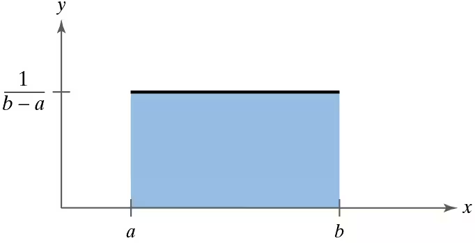
The probability density function of a uniform distribution is

on the interval from (x=a) to (x=b). For any value of x less than a or greater than b, y=0 . In Exercises 59 and 60, use this information.
For two values c and d, where a ≤ c < d ≤ b, the probability that x lies between c and d is equal to the area under the curve between c and d, as shown below.
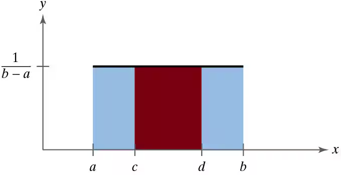
So, the area of the red region equals the probability that x lies between c and d. For a uniform distribution from (a=1) to (b=25) , find the probability that
a. x lies between 2 and 8.
 Verified step by step guidance
1
Step 1: Understand the uniform distribution. A uniform distribution is a continuous probability distribution where all values between two bounds (a and b) are equally likely. The probability density function (PDF) is constant and given by y = 1 / (b - a).
Step 2: Identify the bounds of the distribution. In this problem, the uniform distribution is defined between a = 1 and b = 25. The height of the rectangle (PDF value) is y = 1 / (b - a), which simplifies to y = 1 / (25 - 1).
Step 3: Recognize that the probability of x lying between two values (c and d) is equal to the area under the curve between c and d. This area is a rectangle with width (d - c) and height y = 1 / (b - a).
Step 4: Substitute the values for c and d. Here, c = 2 and d = 8. The width of the rectangle is (d - c) = (8 - 2). The height remains y = 1 / (25 - 1).
Step 5: Calculate the area of the rectangle, which represents the probability. The formula for the area is Area = width Ă— height = (d - c) Ă— (1 / (b - a)). Substitute the values to find the probability that x lies between 2 and 8.
Verified video answer for a similar problem:This video solution was recommended by our tutors as helpful for the problem above
Video duration:
1mWas this helpful?
Key Concepts
Here are the essential concepts you must grasp in order to answer the question correctly.
Uniform Distribution
A uniform distribution is a type of probability distribution where all outcomes are equally likely within a specified range, defined by two parameters, a and b. The probability density function (PDF) is constant between these two values, resulting in a rectangular shape when graphed. This means that for any value of x within the interval [a, b], the likelihood of occurrence is the same.
Recommended video:
Guided course

 06:38
06:38Intro to Frequency Distributions
Probability Density Function (PDF)
The probability density function for a uniform distribution is given by the formula y = 1 / (b - a) for a ≤ x ≤ b, and y = 0 otherwise. This function describes the height of the rectangle in the graph of the uniform distribution, where the area under the curve represents the probability of the random variable falling within a specific interval. The total area under the PDF over the interval [a, b] equals 1.
Recommended video:
 5:37
5:37Introduction to Probability
Area Under the Curve
In the context of a uniform distribution, the probability that a random variable x lies between two values c and d (where a ≤ c < d ≤ b) is determined by the area under the curve of the PDF between these two points. Since the PDF is constant, this area can be calculated as the product of the width (d - c) and the height (1 / (b - a)), providing a straightforward method to find probabilities for intervals within the distribution.
Recommended video:
Guided course
 08:50
08:50Z-Scores from Probabilities
 9:47m
9:47mWatch next
Master Finding Standard Normal Probabilities using z-Table with a bite sized video explanation from Patrick
Start learning

