Performing a Chi-Square Goodness-of-Fit Test

Question

In Exercises 7–16, (d) decide whether to reject or fail to reject the null hypothesis.

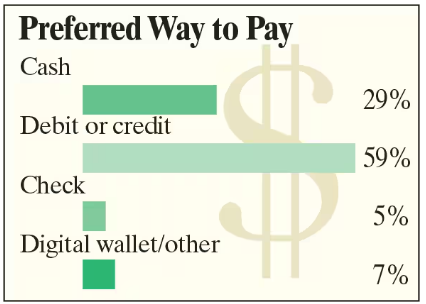
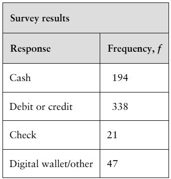
Ways to Pay A financial analyst claims that the distribution of people’s preferences on how to pay for goods is different from the distribution shown in the figure. You randomly select 600 people and record their preferences on how to pay for goods. The table shows the results. At α=0.01, test the financial analyst’s claim. (Adapted from Travis Credit Union)

Accepted Answer

All right. Hello, everyone. So this question says, a researcher claims the distribution of people's preferred grocery shopping methods has changed from a past survey. According to the past survey, the distribution was in-store shopping 50%, online pick up 20%, home delivery 15%, and subscription service, 15%. To test this claim, a sample of 400 people was surveyed with the following results. Decide whether to reject or fail to reject the null hypothesis if alpha equals 0.05. And here we have 4 different answer choices labeled A through D. So To decide whether or not we reject or fail to reject the null hypothesis, we first have to calculate the chi square test statistic and compare this to a critical value. So Recall that the chi square test statistic is equal to the sum of. All differences between observed and expected frequencies squared. Divided by the expected frequency. So let's break down what this means. The expected frequency would be. The frequency for each category based off of the prior survey's data. The observed frequency would be the survey results given to us in the tape. So Based on the data from the past survey, the expected frequency is equal to. The percentage for each category expressed at the decimal multiplied by the sample size. So for in-store shopping, for example, the expected frequency is 0.5, multiplied by 400, which gives you 200. So for online pickup, that's 0.2 multiplied by 400. And that's 80 And then for home delivery and a subscription service, they would both be equal to 0.15. Oops. Did not mean to do that. But it would be 0.15. Multiplied by 400. And that equals 60 So now To illustrate the calculation. That you have to make for each category. Let's use in-store shopping as an example. So based on the new survey, the observed frequency for in-store shopping was 180. So what you're going to do first is take the observed frequency, 180, and subtract the expected frequency. So that's again for in-store shopping, 180 subtracted by 200. And this difference is equal to -20. So now, you are to square the difference between observed and expected frequency, and then divide the square of the difference by the expected frequency. So here that's -20 squad, divided by 200. And that Gives you minus or O subtracted by E squared divided by E. So for this first category of in-store shopping, that value is 2.00. When you repeat these calculations for the, for the remaining three categories, the remaining values are as follows. For online pickup, that's 1.25. For home delivery, it is 1.67. And for subscription service, it's 0.00. So now to find the critical, or excuse me, the test statistic, you would find the sum of all of these values to the right side of the screen that were obtained. And this sum is equal to 4.92. 4.92 is therefore your test statistic. So now, we have to find the critical value to compare our test statistic to. Here, we first need the degrees of freedom. Which in this case would be equal to. The 4 different shopping methods included in the survey, subtracted by 1, which equals 3. So our critical chi square value. At alpha equals 0.05, and with 3 degrees of freedom. is equal to 7.815. Because our test statistic, 4.92 is less than the critical value, 7.815, we fail to reject the null hypothesis. And there you have it. So based on the information that we just found, This corresponds to option C in the multiple choice, making that the correct answer. And so with that being said, thank you so very much for watching, and I hope you found this helpful.

��app

Watch next

����app

Watch next

��app