2. Describing Data with Tables and Graphs
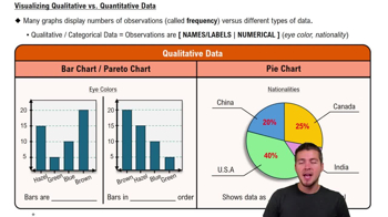
Visualizing Qualitative vs. Quantitative Data
Problem 6.CRE.2d
Textbook Question
In Exercises 1 and 2, use the following wait times (minutes) at 10:00 AM for the Tower of Terror ride at Disney World (from Data Set 33 ŌĆ£Disney World Wait TimesŌĆØ in Appendix B).
35 35 20 50 95 75 45 50 30 35 30 30
d. The accompanying normal quantile plot is obtained by using all 50 wait times at 10:00 AM for the Tower of Terror ride at Disney World. Based on this normal quantile plot, do the sample data appear to be from a normally distributed population?

 Verified step by step guidance
1
Step 1: Understand the purpose of a normal quantile plot. A normal quantile plot is used to assess whether a dataset follows a normal distribution. If the points in the plot closely follow a straight line, the data is likely from a normally distributed population.
Step 2: Examine the provided normal quantile plot. The plot shows the wait times (minutes) for the Tower of Terror ride at 10:00 AM, with Z-scores on the vertical axis and wait times on the horizontal axis. The orange line represents the expected linear relationship if the data were perfectly normal.
Step 3: Analyze the alignment of the data points with the orange line. In the plot, most of the data points closely follow the orange line, indicating a strong linear relationship. However, there are slight deviations at the extremes (lower and upper ends of the wait times).
Step 4: Interpret the deviations. The slight deviations at the extremes suggest that the data may not be perfectly normal, but the overall alignment with the line indicates that the data is approximately normal.
Step 5: Conclude based on the analysis. Based on the normal quantile plot, the sample data appears to be from a population that is approximately normally distributed, with minor deviations at the extremes.
Verified video answer for a similar problem:This video solution was recommended by our tutors as helpful for the problem above
Video duration:
2mWas this helpful?

 4:39m
4:39mWatch next
Master Visualizing Qualitative vs. Quantitative Data with a bite sized video explanation from Patrick
Start learning