2. Describing Data with Tables and Graphs
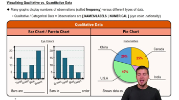
Visualizing Qualitative vs. Quantitative Data
Problem 10.5.6
Textbook Question
Finding the Best Model
In Exercises 5–16, construct a scatterplot and identify the mathematical model that best fits the given data. Assume that the model is to be used only for the scope of the given data, and consider only linear, quadratic, logarithmic, exponential, and power models.
Dirt Cheap The Cherry Hill Construction company in Branford, CT sells screened topsoil by the “yard,” which is actually a cubic yard. Let the variable x be the length (yd) of each side of a cube of screened topsoil. The table below lists the values of x along with the corresponding cost (dollars).

 Verified step by step guidance
1
Step 1: Begin by plotting the given data points on a scatterplot. Use the variable x (length of each side of the cube in yards) as the independent variable on the x-axis and the cost (in dollars) as the dependent variable on the y-axis.
Step 2: Observe the pattern of the data points on the scatterplot. Determine whether the relationship between x and cost appears to be linear, quadratic, logarithmic, exponential, or power-based. Look for trends such as curvature, rapid growth, or proportional scaling.
Step 3: Fit each of the potential models (linear, quadratic, logarithmic, exponential, and power) to the data using regression techniques. For example, use the least squares method to calculate the coefficients for each model.
Step 4: Evaluate the goodness-of-fit for each model using statistical measures such as the coefficient of determination (R²). The model with the highest R² value is likely the best fit for the data.
Step 5: Once the best-fitting model is identified, write down its mathematical equation. Ensure that the model is only used within the scope of the given data, as extrapolation beyond the provided range may lead to inaccuracies.
Verified video answer for a similar problem:This video solution was recommended by our tutors as helpful for the problem above
Video duration:
3mWas this helpful?

 4:39m
4:39mWatch next
Master Visualizing Qualitative vs. Quantitative Data with a bite sized video explanation from Patrick
Start learning