6. Normal Distribution and Continuous Random Variables
Standard Normal Distribution
Problem 6.1.25
Textbook Question
Standard Normal Distribution. In Exercises 17ŌĆō36, assume that a randomly selected subject is given a bone density test. Those test scores are normally distributed with a mean of 0 and a standard deviation of 1. In each case, draw a graph, then find the probability of the given bone density test scores. If using technology instead of Table A-2, round answers to four decimal places.
Between 1.50 and 2.00
 Verified step by step guidance
1
Step 1: Understand the problem. The bone density test scores follow a standard normal distribution, which means the mean (╬╝) is 0 and the standard deviation (Žā) is 1. We are tasked with finding the probability that a score lies between 1.50 and 2.00.
Step 2: Represent the problem graphically. Draw a standard normal distribution curve (bell-shaped curve) with the mean at 0. Mark the points 1.50 and 2.00 on the horizontal axis. Shade the area under the curve between these two points, as this represents the probability we are trying to find.
Step 3: Use the cumulative distribution function (CDF) of the standard normal distribution to find the probabilities corresponding to the z-scores of 1.50 and 2.00. The CDF gives the probability that a value is less than or equal to a given z-score. Denote these probabilities as P(Z Ōēż 2.00) and P(Z Ōēż 1.50).
Step 4: Calculate the probability of the range by subtracting the smaller cumulative probability from the larger one. Specifically, compute P(1.50 Ōēż Z Ōēż 2.00) = P(Z Ōēż 2.00) - P(Z Ōēż 1.50).
Step 5: If using technology (e.g., a calculator or statistical software), input the z-scores 1.50 and 2.00 into the standard normal distribution function to find the corresponding cumulative probabilities. Subtract the results as described in Step 4 to obtain the final probability.
Verified video answer for a similar problem:This video solution was recommended by our tutors as helpful for the problem above
Video duration:
2mWas this helpful?
Key Concepts
Here are the essential concepts you must grasp in order to answer the question correctly.
Standard Normal Distribution
The standard normal distribution is a special case of the normal distribution where the mean is 0 and the standard deviation is 1. It is represented by the Z-score, which indicates how many standard deviations an element is from the mean. This distribution is symmetric and bell-shaped, making it useful for calculating probabilities and percentiles for normally distributed data.
Recommended video:
Guided course

 09:47
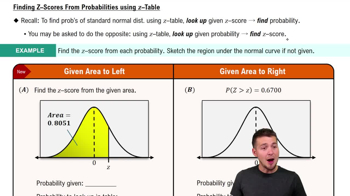
09:47Finding Standard Normal Probabilities using z-Table
Z-scores
A Z-score is a statistical measurement that describes a value's relationship to the mean of a group of values. It is calculated by subtracting the mean from the value and then dividing by the standard deviation. Z-scores allow for the comparison of scores from different normal distributions by standardizing them, making it easier to find probabilities using the standard normal distribution.
Recommended video:
Guided course
 06:31
06:31Z-Scores From Given Probability - TI-84 (CE) Calculator
Probability and Area Under the Curve
In the context of the normal distribution, the probability of a score falling within a certain range is represented by the area under the curve of the distribution graph. To find this probability, one can use Z-scores to determine the corresponding areas from the standard normal distribution table or technology. The total area under the curve equals 1, representing the total probability of all possible outcomes.
Recommended video:
 5:37
5:37Introduction to Probability
 9:47m
9:47mWatch next
Master Finding Standard Normal Probabilities using z-Table with a bite sized video explanation from Patrick
Start learning