6. Normal Distribution and Continuous Random Variables
Standard Normal Distribution
Problem 6.4.7a
Textbook Question
Using the Central Limit Theorem. In Exercises 5–8, assume that the amounts of weight that male college students gain during their freshman year are normally distributed with a mean of 1.2 kg and a standard deviation of 4.9 kg (based on Data Set 13 “Freshman 15” in Appendix B).
a. If 1 male college student is randomly selected, find the probability that he gains between 0 kg and 3 kg during freshman year.
 Verified step by step guidance
1
Step 1: Identify the given parameters. The problem states that the weight gain is normally distributed with a mean (μ) of 1.2 kg and a standard deviation (σ) of 4.9 kg. We are tasked with finding the probability that a randomly selected male college student gains between 0 kg and 3 kg.
Step 2: Standardize the values of 0 kg and 3 kg using the z-score formula: z = (X - μ) / σ. For X = 0 kg, calculate z₁ = (0 - 1.2) / 4.9. For X = 3 kg, calculate z₂ = (3 - 1.2) / 4.9.
Step 3: Use the z-scores calculated in Step 2 to find the corresponding probabilities from the standard normal distribution table (or use statistical software). Let P(z‚ÇÅ) represent the cumulative probability for z‚ÇÅ and P(z‚ÇÇ) represent the cumulative probability for z‚ÇÇ.
Step 4: To find the probability that the weight gain is between 0 kg and 3 kg, subtract the cumulative probability for z₁ from the cumulative probability for z₂. Mathematically, this is expressed as P(0 ≤ X ≤ 3) = P(z₂) - P(z₁).
Step 5: Interpret the result. The value obtained in Step 4 represents the probability that a randomly selected male college student gains between 0 kg and 3 kg during their freshman year.
Verified video answer for a similar problem:This video solution was recommended by our tutors as helpful for the problem above
Video duration:
5mWas this helpful?
Key Concepts
Here are the essential concepts you must grasp in order to answer the question correctly.
Central Limit Theorem
The Central Limit Theorem (CLT) states that the distribution of the sample means will approach a normal distribution as the sample size increases, regardless of the original distribution of the population. This theorem is crucial for making inferences about population parameters based on sample statistics, especially when dealing with large samples.
Recommended video:
Guided course

 04:52
04:52Calculating the Mean
Normal Distribution
A normal distribution is a continuous probability distribution characterized by its bell-shaped curve, defined by its mean and standard deviation. In this context, the weights gained by male college students are normally distributed, which allows us to use properties of the normal distribution to calculate probabilities related to weight gain.
Recommended video:
Guided course
 09:47
09:47Finding Standard Normal Probabilities using z-Table
Probability Calculation
Probability calculation involves determining the likelihood of a specific outcome occurring within a defined range. In this scenario, we need to calculate the probability that a randomly selected male college student gains between 0 kg and 3 kg, which requires using the properties of the normal distribution and potentially standardizing the values using the z-score formula.
Recommended video:
Guided course
 07:09
07:09Probability From Given Z-Scores - TI-84 (CE) Calculator
 9:47m
9:47mWatch next
Master Finding Standard Normal Probabilities using z-Table with a bite sized video explanation from Patrick
Start learning