6. Normal Distribution and Continuous Random Variables
Standard Normal Distribution
Problem 5.Q.4c
Textbook Question
The random variable x is normally distributed with the given parameters. Find each probability.
c. μ = 5.5, σ ≈ 0.08, P(5.36 < x < 5.64)
 Verified step by step guidance
1
Step 1: Recognize that the problem involves a normal distribution with mean (μ) = 5.5 and standard deviation (σ) ≈ 0.08. The goal is to find the probability that the random variable x lies between 5.36 and 5.64, i.e., P(5.36 < x < 5.64).
Step 2: Standardize the values 5.36 and 5.64 using the z-score formula: z = (x - μ) / σ. For x = 5.36, calculate z₁ = (5.36 - 5.5) / 0.08. For x = 5.64, calculate z₂ = (5.64 - 5.5) / 0.08.
Step 3: Use a standard normal distribution table or a statistical software to find the cumulative probabilities corresponding to z₁ and z₂. Let Φ(z₁) represent the cumulative probability for z₁ and Φ(z₂) represent the cumulative probability for z₂.
Step 4: Compute the probability P(5.36 < x < 5.64) by subtracting the cumulative probability for z₁ from the cumulative probability for z₂: P(5.36 < x < 5.64) = Φ(z₂) - Φ(z₁).
Step 5: Interpret the result as the probability that the random variable x falls within the specified range, based on the standard normal distribution.
Verified video answer for a similar problem:This video solution was recommended by our tutors as helpful for the problem above
Video duration:
2mWas this helpful?
Key Concepts
Here are the essential concepts you must grasp in order to answer the question correctly.
Normal Distribution
The normal distribution is a continuous probability distribution characterized by its bell-shaped curve, defined by its mean (μ) and standard deviation (σ). It is symmetric around the mean, meaning that approximately 68% of the data falls within one standard deviation from the mean, and about 95% falls within two standard deviations. This distribution is fundamental in statistics as many real-world phenomena tend to follow this pattern.
Recommended video:

 06:23
06:23Using the Normal Distribution to Approximate Binomial Probabilities
Standard Normal Distribution
The standard normal distribution is a special case of the normal distribution where the mean is 0 and the standard deviation is 1. To find probabilities for any normal distribution, we can convert the values to z-scores using the formula z = (x - μ) / σ. This transformation allows us to use standard normal distribution tables or software to find probabilities associated with any normal distribution.
Recommended video:
Guided course
 09:47
09:47Finding Standard Normal Probabilities using z-Table
Probability Calculation
To calculate the probability of a random variable falling within a specific range in a normal distribution, we find the z-scores for the endpoints of the range and then use the standard normal distribution to determine the area under the curve between these z-scores. This area represents the probability that the random variable falls within the specified range, which can be found using cumulative distribution functions or z-tables.
Recommended video:
Guided course
 07:09
07:09Probability From Given Z-Scores - TI-84 (CE) Calculator
 9:47m
9:47mWatch next
Master Finding Standard Normal Probabilities using z-Table with a bite sized video explanation from Patrick
Start learning