Table of contents
- 1. Intro to Stats and Collecting Data55m
- 2. Describing Data with Tables and Graphs1h 55m
- 3. Describing Data Numerically1h 45m
- 4. Probability2h 16m
- 5. Binomial Distribution & Discrete Random Variables2h 33m
- 6. Normal Distribution and Continuous Random Variables1h 38m
- 7. Sampling Distributions & Confidence Intervals: Mean1h 3m
- 8. Sampling Distributions & Confidence Intervals: Proportion1h 12m
- 9. Hypothesis Testing for One Sample1h 1m
- 10. Hypothesis Testing for Two Samples2h 8m
- 11. Correlation48m
- 12. Regression1h 4m
- 13. Chi-Square Tests & Goodness of Fit1h 20m
- 14. ANOVA1h 0m
1. Intro to Stats and Collecting Data
Intro to Stats
Problem 10.2.12a
Textbook Question
Effects of Clusters Refer to the Minitab-generated scatterplot given in Exercise 10 of Section 10-1.
a. Using the pairs of values for all 8 points, find the equation of the regression line.
 Verified step by step guidance
1
Step 1: Identify the data points. Extract the pairs of values (x, y) for all 8 points from the scatterplot provided in Exercise 10 of Section 10-1.a. These pairs represent the independent variable (x) and the dependent variable (y).
Step 2: Calculate the means of x and y. Use the formulas \( \bar{x} = \frac{\sum x}{n} \) and \( \bar{y} = \frac{\sum y}{n} \), where \( n \) is the number of data points (in this case, 8).
Step 3: Compute the slope (b1) of the regression line. Use the formula \( b_1 = \frac{\sum (x_i - \bar{x})(y_i - \bar{y})}{\sum (x_i - \bar{x})^2} \), where \( x_i \) and \( y_i \) are the individual data points, and \( \bar{x} \) and \( \bar{y} \) are the means calculated in Step 2.
Step 4: Calculate the y-intercept (b0) of the regression line. Use the formula \( b_0 = \bar{y} - b_1 \bar{x} \), substituting the values of \( \bar{y} \), \( \bar{x} \), and \( b_1 \) from the previous steps.
Step 5: Write the equation of the regression line. Combine the slope \( b_1 \) and the y-intercept \( b_0 \) into the equation \( y = b_0 + b_1x \). This is the final form of the regression line equation.
 Verified video answer for a similar problem:
This video solution was recommended by our tutors as helpful for the problem above
Video duration:
2mPlay a video:
Was this helpful?
Key Concepts
Here are the essential concepts you must grasp in order to answer the question correctly.
Regression Line
A regression line is a statistical tool used to model the relationship between two variables by fitting a linear equation to observed data. The equation typically takes the form y = mx + b, where m represents the slope and b the y-intercept. This line helps predict the value of the dependent variable based on the independent variable, making it essential for understanding trends in scatterplots.
Recommended video:
Guided course

Correlation Coefficient
Scatterplot
A scatterplot is a graphical representation of two variables, where each point represents an observation in the dataset. It allows for visual assessment of the relationship between the variables, indicating patterns, trends, or correlations. Analyzing a scatterplot is crucial for determining the appropriateness of a regression analysis and understanding the data's distribution.
Recommended video:
Guided course

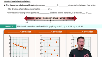
Scatterplots & Intro to Correlation
Least Squares Method
The least squares method is a mathematical approach used to determine the best-fitting line for a set of data points in regression analysis. It minimizes the sum of the squares of the vertical distances (residuals) between the observed values and the values predicted by the regression line. This method ensures that the regression line is as close as possible to all data points, providing a reliable model for predictions.
Recommended video:

Constructing Confidence Intervals for Proportions

 2:13m
2:13mWatch next
Master Introduction to Statistics Channel with a bite sized video explanation from Patrick
Start learning


