6. Normal Distribution and Continuous Random Variables
Standard Normal Distribution
Problem 5.5.27c
Textbook Question
Daily Commute About 83% of U.S. employees drive their own vehicle to work. You randomly select a sample of U.S. employees. Find the probability that more than 100 of the employees drive their own vehicle to work. (Source: U.S. Bureau of Labor Statistics)
c. You select 150 U.S. employees.
 Verified step by step guidance
1
Step 1: Identify the type of probability distribution to use. Since we are dealing with a proportion (83%) and a sample size (n = 150), this problem involves a binomial distribution. However, for large sample sizes, the binomial distribution can be approximated by a normal distribution. Check if the normal approximation is valid by ensuring that both np and n(1-p) are greater than 5.
Step 2: Calculate the mean (╬╝) and standard deviation (Žā) of the binomial distribution. The mean is given by ╬╝ = np, and the standard deviation is given by Žā = ŌłÜ(np(1-p)), where n is the sample size and p is the proportion of employees who drive their own vehicle to work.
Step 3: Convert the problem to a normal distribution approximation. To find the probability that more than 100 employees drive their own vehicle to work, calculate the z-score using the formula z = (X - ╬╝) / Žā, where X is the value of interest (100 in this case).
Step 4: Use the z-score to find the corresponding probability. Look up the z-score in a standard normal distribution table or use statistical software to find the cumulative probability up to the z-score. Subtract this cumulative probability from 1 to find the probability of more than 100 employees driving their own vehicle to work.
Step 5: Interpret the result. The final probability represents the likelihood that more than 100 employees in the sample of 150 drive their own vehicle to work. Ensure the interpretation aligns with the context of the problem.
Verified video answer for a similar problem:This video solution was recommended by our tutors as helpful for the problem above
Video duration:
10mWas this helpful?
Key Concepts
Here are the essential concepts you must grasp in order to answer the question correctly.
Probability
Probability is a measure of the likelihood that a particular event will occur, expressed as a number between 0 and 1. In this context, it helps determine the chance that more than 100 out of 150 randomly selected employees drive their own vehicle to work, given that 83% of employees do so.
Recommended video:

 5:37
5:37Introduction to Probability
Binomial Distribution
The binomial distribution models the number of successes in a fixed number of independent Bernoulli trials, each with the same probability of success. Here, it applies to the scenario of selecting 150 employees, where each employee either drives their own vehicle (success) or does not (failure), allowing us to calculate the probability of observing more than 100 successes.
Recommended video:
Guided course
 03:28
03:28Mean & Standard Deviation of Binomial Distribution
Normal Approximation
The normal approximation to the binomial distribution is used when the sample size is large, allowing for easier calculations. Since the sample size of 150 is sufficiently large, we can approximate the binomial distribution with a normal distribution to find the probability of more than 100 employees driving their own vehicle.
Recommended video:
 06:23
06:23Using the Normal Distribution to Approximate Binomial Probabilities
 9:47m
9:47mWatch next
Master Finding Standard Normal Probabilities using z-Table with a bite sized video explanation from Patrick
Start learning